Data sets

Let us assume that we took several pictures with our camera. Typically, these photos are simply stored as image files without any further description about the content of the images. We can understand this collection of photos as a data set and since we have no further description of the individual images, we speak about an unlabeled data set. By augmenting the unlabeled data set with interesting information, we obtain a labeled data set. "Interesting" in this context depends on the goal we want to achieve within our use case. For example, it could be interesting to know the content of the images, then we might label the images with descriptions like beach, person, landscape, animal, and so on. Or we would like to know whether the image was taken at day or night, so we label each image with this information, or possibly we are just interested in the number of persons in an image.

Simply speaking, a data set is a collection of data (and of course not restricted to images), labeled data is a data set that augments each data point with some meaningful tag(s) and in unlabeled data this tag is missing.

Supervised and unsupervised learning

In unsupervised learning, we basically try to find patterns within unlabeled data. In supervised learning, we try to map an input (features) to an output (labels) and thus require labeled data. Supervised learning boils down to prediction tasks like classification or regression.

MNIST data set

To demonstrate some applications of unsupervised and supervised machine learning algorithms we will have a look at the famous MNIST data set. This data set consists of 70.000 images of handwritten digits and additionally a label that tells the digit which is displayed in the individual images.

The data set looks like this:

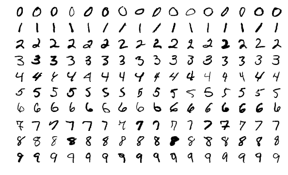
But let us dive into this data set by ourselves. Luckily, there is a package MLDatasets.jl that makes it easy to load this data set (and also many others) into Julia. When you are loading the data set for the first time, you might need to confirm the download within the prompt.

julia> using MLDatasets

julia> mnist_data = MNIST()
dataset MNIST:
  metadata    =>    Dict{String, Any} with 3 entries
  split       =>    :train
  features    =>    28×28×60000 Array{Float32, 3}
  targets     =>    60000-element Vector{Int64}

Apparently, mnist_data comes with some meta information and when having a look at the help for MNIST() we get the (incomplete) description:

•  metadata: A dictionary containing additional information on the dataset.

    •  features: An array storing the data features.

    •  targets: An array storing the targets for supervised learning.

    •  split.

We are mainly interested in features where we find the $28 \times 28$ images of handwritten digits and at targets where we find the according labels. The split tells at which part of the data set we are looking. Especially for supervised learning we need a way to test our model with previously unseen data. So usually - in the context of supervised learning - data sets are split into two parts: a training data set which is used for training or fitting a model and a test data set which is used to evaluate the quality of the model. For some algorithms, we often introduce a third data split: a validation data set which is used to evaluate a model while tuning hyper parameters or to stop training before running into overfitting. But for this workshop we will stick to training and test data set. The manual also states that MNIST() is setting split to :train by default.

julia> df_train = MNIST(:train)

dataset MNIST:
  metadata    =>    Dict{String, Any} with 3 entries
  split       =>    :train
  features    =>    28×28×60000 Array{Float32, 3}
  targets     =>    60000-element Vector{Int64}

julia> df_test = MNIST(:test)
dataset MNIST:
  metadata    =>    Dict{String, Any} with 3 entries
  split       =>    :test
  features    =>    28×28×10000 Array{Float32, 3}
  targets     =>    10000-element Vector{Int64}

julia> using ImageInTerminal, ImageShow

julia> nrImgs = 5
5

julia> convert2image(df_train, 1:nrImgs)

julia> convert2image(df_test, 1:nrImgs)

Most learning algorithms require the data to be in tabular form, but the features are currently given as a three-dimensional array. So our next goal is to reshape the training and test data from an 28×28×NR_IMAGES array to a 784×NR_IMAGES array.

julia> X_train = reshape(df_train.features, (28 * 28, :))'
60000×784 adjoint(::Matrix{Float32}) with eltype Float32:
 0.0  0.0  0.0  0.0  0.0  0.0  0.0  0.0  0.0  0.0  0.0  0.0  0.0  0.0  0.0  0.0  0.0  0.0  0.0  0.0  0.0  …  0.0  0.0  0.0  0.0  0.0  0.0  0.0  0.0  0.0  0.0  0.0  0.0  0.0  0.0  0.0  0.0  0.0  0.0  0.0  0.0
 0.0  0.0  0.0  0.0  0.0  0.0  0.0  0.0  0.0  0.0  0.0  0.0  0.0  0.0  0.0  0.0  0.0  0.0  0.0  0.0  0.0     0.0  0.0  0.0  0.0  0.0  0.0  0.0  0.0  0.0  0.0  0.0  0.0  0.0  0.0  0.0  0.0  0.0  0.0  0.0  0.0
 0.0  0.0  0.0  0.0  0.0  0.0  0.0  0.0  0.0  0.0  0.0  0.0  0.0  0.0  0.0  0.0  0.0  0.0  0.0  0.0  0.0     0.0  0.0  0.0  0.0  0.0  0.0  0.0  0.0  0.0  0.0  0.0  0.0  0.0  0.0  0.0  0.0  0.0  0.0  0.0  0.0
 0.0  0.0  0.0  0.0  0.0  0.0  0.0  0.0  0.0  0.0  0.0  0.0  0.0  0.0  0.0  0.0  0.0  0.0  0.0  0.0  0.0     0.0  0.0  0.0  0.0  0.0  0.0  0.0  0.0  0.0  0.0  0.0  0.0  0.0  0.0  0.0  0.0  0.0  0.0  0.0  0.0
 0.0  0.0  0.0  0.0  0.0  0.0  0.0  0.0  0.0  0.0  0.0  0.0  0.0  0.0  0.0  0.0  0.0  0.0  0.0  0.0  0.0     0.0  0.0  0.0  0.0  0.0  0.0  0.0  0.0  0.0  0.0  0.0  0.0  0.0  0.0  0.0  0.0  0.0  0.0  0.0  0.0
 0.0  0.0  0.0  0.0  0.0  0.0  0.0  0.0  0.0  0.0  0.0  0.0  0.0  0.0  0.0  0.0  0.0  0.0  0.0  0.0  0.0  …  0.0  0.0  0.0  0.0  0.0  0.0  0.0  0.0  0.0  0.0  0.0  0.0  0.0  0.0  0.0  0.0  0.0  0.0  0.0  0.0
 ⋮                        ⋮                        ⋮                        ⋮                        ⋮    ⋱       ⋮                        ⋮                        ⋮                        ⋮              
 0.0  0.0  0.0  0.0  0.0  0.0  0.0  0.0  0.0  0.0  0.0  0.0  0.0  0.0  0.0  0.0  0.0  0.0  0.0  0.0  0.0  …  0.0  0.0  0.0  0.0  0.0  0.0  0.0  0.0  0.0  0.0  0.0  0.0  0.0  0.0  0.0  0.0  0.0  0.0  0.0  0.0
 0.0  0.0  0.0  0.0  0.0  0.0  0.0  0.0  0.0  0.0  0.0  0.0  0.0  0.0  0.0  0.0  0.0  0.0  0.0  0.0  0.0     0.0  0.0  0.0  0.0  0.0  0.0  0.0  0.0  0.0  0.0  0.0  0.0  0.0  0.0  0.0  0.0  0.0  0.0  0.0  0.0
 0.0  0.0  0.0  0.0  0.0  0.0  0.0  0.0  0.0  0.0  0.0  0.0  0.0  0.0  0.0  0.0  0.0  0.0  0.0  0.0  0.0     0.0  0.0  0.0  0.0  0.0  0.0  0.0  0.0  0.0  0.0  0.0  0.0  0.0  0.0  0.0  0.0  0.0  0.0  0.0  0.0
 0.0  0.0  0.0  0.0  0.0  0.0  0.0  0.0  0.0  0.0  0.0  0.0  0.0  0.0  0.0  0.0  0.0  0.0  0.0  0.0  0.0     0.0  0.0  0.0  0.0  0.0  0.0  0.0  0.0  0.0  0.0  0.0  0.0  0.0  0.0  0.0  0.0  0.0  0.0  0.0  0.0
 0.0  0.0  0.0  0.0  0.0  0.0  0.0  0.0  0.0  0.0  0.0  0.0  0.0  0.0  0.0  0.0  0.0  0.0  0.0  0.0  0.0     0.0  0.0  0.0  0.0  0.0  0.0  0.0  0.0  0.0  0.0  0.0  0.0  0.0  0.0  0.0  0.0  0.0  0.0  0.0  0.0

julia> X_test = reshape(df_test.features, (28 * 28, :))'
10000×784 adjoint(::Matrix{Float32}) with eltype Float32:
 0.0  0.0  0.0  0.0  0.0  0.0  0.0  0.0  0.0  0.0  0.0  0.0  0.0  0.0  0.0  0.0  0.0  0.0  0.0  0.0  0.0  …  0.0  0.0  0.0  0.0  0.0  0.0  0.0  0.0  0.0  0.0  0.0  0.0  0.0  0.0  0.0  0.0  0.0  0.0  0.0  0.0
 0.0  0.0  0.0  0.0  0.0  0.0  0.0  0.0  0.0  0.0  0.0  0.0  0.0  0.0  0.0  0.0  0.0  0.0  0.0  0.0  0.0     0.0  0.0  0.0  0.0  0.0  0.0  0.0  0.0  0.0  0.0  0.0  0.0  0.0  0.0  0.0  0.0  0.0  0.0  0.0  0.0
 0.0  0.0  0.0  0.0  0.0  0.0  0.0  0.0  0.0  0.0  0.0  0.0  0.0  0.0  0.0  0.0  0.0  0.0  0.0  0.0  0.0     0.0  0.0  0.0  0.0  0.0  0.0  0.0  0.0  0.0  0.0  0.0  0.0  0.0  0.0  0.0  0.0  0.0  0.0  0.0  0.0
 0.0  0.0  0.0  0.0  0.0  0.0  0.0  0.0  0.0  0.0  0.0  0.0  0.0  0.0  0.0  0.0  0.0  0.0  0.0  0.0  0.0     0.0  0.0  0.0  0.0  0.0  0.0  0.0  0.0  0.0  0.0  0.0  0.0  0.0  0.0  0.0  0.0  0.0  0.0  0.0  0.0
 0.0  0.0  0.0  0.0  0.0  0.0  0.0  0.0  0.0  0.0  0.0  0.0  0.0  0.0  0.0  0.0  0.0  0.0  0.0  0.0  0.0     0.0  0.0  0.0  0.0  0.0  0.0  0.0  0.0  0.0  0.0  0.0  0.0  0.0  0.0  0.0  0.0  0.0  0.0  0.0  0.0
 0.0  0.0  0.0  0.0  0.0  0.0  0.0  0.0  0.0  0.0  0.0  0.0  0.0  0.0  0.0  0.0  0.0  0.0  0.0  0.0  0.0  …  0.0  0.0  0.0  0.0  0.0  0.0  0.0  0.0  0.0  0.0  0.0  0.0  0.0  0.0  0.0  0.0  0.0  0.0  0.0  0.0
 ⋮                        ⋮                        ⋮                        ⋮                        ⋮    ⋱       ⋮                        ⋮                        ⋮                        ⋮              
 0.0  0.0  0.0  0.0  0.0  0.0  0.0  0.0  0.0  0.0  0.0  0.0  0.0  0.0  0.0  0.0  0.0  0.0  0.0  0.0  0.0  …  0.0  0.0  0.0  0.0  0.0  0.0  0.0  0.0  0.0  0.0  0.0  0.0  0.0  0.0  0.0  0.0  0.0  0.0  0.0  0.0
 0.0  0.0  0.0  0.0  0.0  0.0  0.0  0.0  0.0  0.0  0.0  0.0  0.0  0.0  0.0  0.0  0.0  0.0  0.0  0.0  0.0     0.0  0.0  0.0  0.0  0.0  0.0  0.0  0.0  0.0  0.0  0.0  0.0  0.0  0.0  0.0  0.0  0.0  0.0  0.0  0.0
 0.0  0.0  0.0  0.0  0.0  0.0  0.0  0.0  0.0  0.0  0.0  0.0  0.0  0.0  0.0  0.0  0.0  0.0  0.0  0.0  0.0     0.0  0.0  0.0  0.0  0.0  0.0  0.0  0.0  0.0  0.0  0.0  0.0  0.0  0.0  0.0  0.0  0.0  0.0  0.0  0.0
 0.0  0.0  0.0  0.0  0.0  0.0  0.0  0.0  0.0  0.0  0.0  0.0  0.0  0.0  0.0  0.0  0.0  0.0  0.0  0.0  0.0     0.0  0.0  0.0  0.0  0.0  0.0  0.0  0.0  0.0  0.0  0.0  0.0  0.0  0.0  0.0  0.0  0.0  0.0  0.0  0.0
 0.0  0.0  0.0  0.0  0.0  0.0  0.0  0.0  0.0  0.0  0.0  0.0  0.0  0.0  0.0  0.0  0.0  0.0  0.0  0.0  0.0     0.0  0.0  0.0  0.0  0.0  0.0  0.0  0.0  0.0  0.0  0.0  0.0  0.0  0.0  0.0  0.0  0.0  0.0  0.0  0.0

When using different algorithms, we always have to keep in mind in which format and shape our data is stored. Different algorithms have different requirements. Sometimes observations have to be stored row wise (each observation in a separate row), sometimes they have to be stored column wise. Some algorithms require a Matrix and others a DataFrame.

Images

In the previous part we used MLDatasets in order to load a dataset consisting of images. Now you might want to prepare your custom dataset consisting of raw image files. You can load most images using FileIO.jl with ImageIO.jl.

julia> using FileIO, ImageIO, Downloads

julia> tmpfile = Downloads.download("https://upload.wikimedia.org/wikipedia/en/7/7d/Lenna_%28test_image%29.png");

julia> img = FileIO.load(tmpfile);

julia> typeof(img)
Matrix{RGB{N0f8}} (alias for Array{RGB{Normed{UInt8, 8}}, 2})

julia> img[1,1]
RGB{N0f8}(0.886,0.537,0.49)

Here we see that the image does not consist of floating point numbers, since RGB images usually only carry 256 distinct values in each channel. Using ImageCore from juliaimages we can however easily convert it

julia> channelview(img) |> size
(3, 512, 512)

julia> float(channelview(img)) |> typeof
Array{Float32, 3}

Thus we get our usual Array{Float32, 3} and with permutedims(float(channelview(img)), [2, 3, 1]) we can e.g. swap the color channel dimension to be last, which is the default for machine learning in Julia. For saving the "processed" image we can use the HDF5 package, which is a standard format like Arrow but for arrays instead of tables.

julia> filename = tempname() * ".hdf5"
"/tmp/jl_cnipopsX8Z.hdf5"

julia> h5open(filename, "w") do f
           f["image", compress=true] = permutedims(float(channelview(img)), [2, 3, 1])
       end;

julia> h5read(filename, "image") |> size
(512, 512, 3)

Custom Datasets and Iterating over Data

The MLUtils.jl package contains utility functions for creating your own custom dataset (that can also be larger than your memory) and to iterate over a subset (minibatches) of your data. For example in order to iterate over the MNIST dataset we can use MLUtils.eachobs, which returns an iterator that one uses with a for loop. We can also use first in order to get the first iteration in order to check what we will be iterating over

julia> first(eachobs(df_train; batchsize=256)) |> typeof
NamedTuple{(:features, :targets), Tuple{Array{Float32, 3}, Vector{Int64}}}

julia> first(eachobs(df_train; batchsize=256)).features |> size
(28, 28, 256)

julia> first(eachobs(df_train; batchsize=256)).targets |> size
(256,)

Here we see that we will receive a NamedTuple of the images and the corresponding labels. Iterating over this dataset and optimize a neural network would then look like the following

for (images, labels) in eachobs(df_train; batchsize=256)
    # calculate loss and gradients and update parameters
end

Additional useful functions might be shuffleobs, splitobs for random shuffling and splitting the data or kfolds for k-fold cross validation.

using MLUtils

struct FakeData
    n::Int
end
MLUtils.numobs(data::FakeData) = data.n
MLUtils.getobs(data::FakeData, idx::AbstractVector{<:Integer} = randn(3, 4, length(idx))