Time series data often exhibits patterns such as trends, seasonality, and cycles. Decomposing a time series into its components can help to better understand the underlying processes.
Time series are usually decomposed into three components:
Trend: \(T_t\), long-term progression of the series (e.g., increasing or decreasing).
Seasonality: \(S_t\), regular patterns that repeat over a fixed period (e.g., daily, weekly, yearly).
Residual: \(I_t\), random noise or irregular component.
Additive models assume that the components add together to form the time series: \[ Y_t = T_t + S_t + I_t \]
Multiplicative models assume that the components multiply together to form the time series: \[ Y_t = T_t \times S_t \times I_t \]
Note
Sometimes, also a fourth component, Cyclic (\(C_t\)), is considered, which represents long-term oscillations that are not of fixed period.
11.1 Examples
This example uses the package statsmodels for time series decomposition.
11.1.1 Imports
Code
import warningsimport numpy as npimport pandas as pdimport plotly.express as pximport plotly.graph_objs as goimport plotly.io as pioimport plotly.subplots as spfrom statsmodels.tsa.seasonal import seasonal_decompose, STL # used for decompositionpio.renderers.default = ("notebook"# set the default plotly renderer to "notebook" (necessary for quarto to render the plots))warnings.filterwarnings("ignore")
11.1.2 Generating Example Data
Code
np.random.seed(42) # for reproducibilitydate_range = pd.date_range(start="2010-01-01", end="2024-12-31", freq="MS")trend =100+0.9* np.arange(len(date_range)) # nonlinear trendseasonality =121* np.sin(np.pi * (date_range.month /12)) # yearly seasonalitynoise = np.random.normal(0, 21, len(date_range)) # random noise at each point# Add outliers with a probability of 0.05outlier_mask = np.random.rand(len(date_range)) <0.05outlier_values = np.random.normal(10, 100, len(date_range)) # large outliersnoise[outlier_mask] += outlier_values[outlier_mask]sales = trend + seasonality + noise # final data as sum of all componentsdf = pd.DataFrame({"Date": date_range, "Sales": sales}).set_index("Date")
fig = px.line(df, y="Sales", title="Sales Over Time")fig.show()
In the above plot, we can see a clear upward trend, but identifying seasonality is more difficult. To support this visual analysis, we add vertical lines at the beginning of each year.
fig = px.line(df, y="Sales", title="Sales Over Time")for year inrange(df.index.year.min(), df.index.year.max() +1): fig.add_vline( x=pd.Timestamp(f"{year}-01-01"), line_dash="dash", line_color="gray", opacity=0.5, )fig.show()
Now it is apparent that there is a yearly seasonal pattern, with peaks around mid-year.
11.1.3 Algorithmic Decomposition
Algorithmic decomposition of a time series into its components is not a trivial task. Many algorithms exist to achieve this, each with its own advantages and disadvantages.
In the following, we use a very simple additive model based on moving averages to decompose our time series. First, the trend is estimated using a moving average with a smaller window size. Then, the detrended series is calculated by subtracting the trend from the original series. The seasonal component is estimated by averaging the values for each season (e.g., each month, year, ..) in the detrended time series. Finally, the residual component is calculated by subtracting both the trend and seasonal components from the original series.
Note that this is a very naive approach and according to the documentation of seasonal_decompose a more sophisticated method should be preferred. However, it is easy to understand and serves well for demonstration purposes.
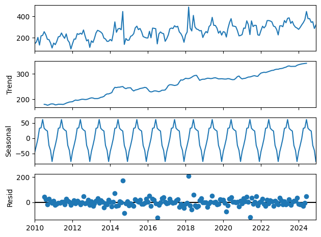
In previous plot, we can see that the estimated values follow the observed values quite closely, indicating that the STL decomposition has effectively captured the underlying patterns in the data. But we can also see some points with larger deviations, which are likely outliers in the original data.
11.1.5 Anomaly Detection
One way to quantify outliers is to apply a threshold to the residuals (e.g., 3 times the standard deviation of the residuals, also known as the 3-sigma rule).