import pandas as pd # used for data handling
import seaborn as sns # used for statistical data visualization
import plotly.express as px # used for performant plotting
import plotly.io as pio # used to set the default plotly renderer
pio.renderers.default = (
"notebook" # set the default plotly renderer to "notebook" (necessary for quarto to render the plots)
)20 Process optimization on sensor data via EDA
In this section, we will have a look at a more realistic example of industrial data.
20.1 Setting the stage
Imagine a manufacturing chain which is dedicated to producing knives with wooden handles. Various machines are interconnected and the process flow is as follows:
- Machine A prepares the steel blade and shaft.
- Machine B applies epoxy to the grip area.
- Machine C inserts the wooden handle material.
- Machine D is a curing oven, hardening the adhesive.
- Machine E coats the knife with protective finish and completes the manufacturing process.
Operators notice that the process is not running as smoothly as expected. The handle is not always properly bonded to the metal piece and sometimes the wood is cracked. They find that the root cause of the issue lies in the epoxy application step of Machine B. Common issues include excessive or insufficient epoxy application, uneven distribution, and occasional poor adhesion to the shaft. One clear economic impact is that these defective products cannot be sold. But there is more to it:
- Waste of material is not sustainable.
- The defect actually already happens in Machine B, but Machines C to E still process the faulty products, leading to further waste and costs, especially since the wooden handle is the most expensive part of the product and the curing oven is very energy-intensive.
Since there is a new department focused on data science, they decide to manually inspect the epoxy application right after Machine B and label the data accordingly. Additionally the machine collects some sensor data in a CSV file. This dataset is given to the data science team and in tight collaboration with the operators the ambitious goal is to:
- Optimize the epoxy application process to reduce defects and waste.
- Human inspection is time-consuming and expensive. Find a way to predict defects occuring in Machine B before the product is handed over to machine C.
Of course, this data science department is us.
20.2 Dataset
The dataset consists of sensor readings of a simulated industrial process and consists of two files:
simulated_machine_data.csvstores the sensor datasimulated_inspection_data.csvstores the human inspection results
The sensor data includes the following features in a 200ms resolution:
air_temperature_C: Ambient air temperature in degrees Celsius.machine_temperature_C: Temperature of the machine in degrees Celsius.pressure_measured_bar: Measured pressure in bar.pressure_setting_bar: Pressure setting in bar.process_speed_mm_s: Set speed of the process in millimeters per second.process_step_index: Index indicating the current step within the process.product_id: Unique identifier for each product. The machine performs three processing steps: moving the nozzle to the shaft, applying epoxy, and blowing out residual epoxy from the nozzle while moving away.timestamp: Timestamp of the sensor reading.
The inspection data includes the product_id and the error_code:
error_code: Code indicating the type of error detected during inspection.product_id: Unique identifier for each product.
They used OK when there was no defect, NOK_1 (excessive epoxy), NOK_2 (insufficient epoxy), NOK_3 (poor adhesion), and NOK_4 (uneven distribution).
20.3 Additional information
The operators state that the epoxy application process is highly sensitive to variations in environmental conditions, such as temperature and humidity. They believe that incorporating additional sensor data, such as humidity levels, could further enhance understanding of the process. Also, the pressure settings are critical, since they directly influence the amount of epoxy applied to the product. The first processing step ensures the correct positioning of the nozzle and the final processing step is supposed to clean the nozzle, preparing it for the next application.
20.4 Exploratory Data Analysis
20.4.1 Loading packages
20.4.2 Loading the dataset
The dataset is available online in the form of two csv files.
It was released at Ehrensperger (2026), but you can also clone the source repository from GitHub.
df_processes = pd.read_csv(
"https://github.com/noxthot/industrial_datascience_sim_machine_knifes/raw/refs/tags/v1.0.2/data/simulated_machine_data.csv"
)
df_inspections = pd.read_csv(
"https://github.com/noxthot/industrial_datascience_sim_machine_knifes/raw/refs/tags/v1.0.2/data/simulated_inspection_data.csv"
)20.4.3 Quick check data integrity
df_processes| nr_iteration | process_step_index | timestamp | air_temperature_C | process_speed_mm_s | pressure_measured_bar | pressure_setting_bar | machine_temperature_C | |
|---|---|---|---|---|---|---|---|---|
| 0 | 0 | 0 | 2024-06-01 21:00:00.000 | 17.411810 | 10 | 14.221200 | 5 | 17.413006 |
| 1 | 0 | 0 | 2024-06-01 21:00:00.200 | 17.411810 | 10 | 10.564433 | 5 | 17.412700 |
| 2 | 0 | 0 | 2024-06-01 21:00:00.400 | 17.411810 | 10 | 10.054016 | 5 | 17.413947 |
| 3 | 0 | 0 | 2024-06-01 21:00:00.600 | 17.411810 | 10 | 10.103557 | 5 | 17.414270 |
| 4 | 0 | 0 | 2024-06-01 21:00:00.800 | 17.411810 | 10 | 11.594134 | 5 | 17.415649 |
| ... | ... | ... | ... | ... | ... | ... | ... | ... |
| 199995 | 4999 | 2 | 2024-06-02 08:06:39.000 | 20.261769 | 20 | 24.946507 | 20 | 45.459340 |
| 199996 | 4999 | 2 | 2024-06-02 08:06:39.200 | 20.261769 | 20 | 26.045240 | 20 | 45.461210 |
| 199997 | 4999 | 2 | 2024-06-02 08:06:39.400 | 20.261769 | 20 | 30.247436 | 20 | 45.459048 |
| 199998 | 4999 | 2 | 2024-06-02 08:06:39.600 | 20.261769 | 20 | 30.317732 | 20 | 45.455973 |
| 199999 | 4999 | 2 | 2024-06-02 08:06:39.800 | 20.261769 | 20 | 27.688261 | 20 | 45.455442 |
200000 rows × 8 columns
df_inspections| timestamp | error_code | |
|---|---|---|
| 0 | 2024-06-01 21:00:10.068501 | OK |
| 1 | 2024-06-01 21:00:20.934694 | OK |
| 2 | 2024-06-01 21:00:25.997543 | OK |
| 3 | 2024-06-01 21:00:36.090388 | OK |
| 4 | 2024-06-01 21:00:44.213738 | OK |
| ... | ... | ... |
| 4995 | 2024-06-02 08:06:10.582952 | OK |
| 4996 | 2024-06-02 08:06:19.236113 | NOK_4 |
| 4997 | 2024-06-02 08:06:25.214726 | OK |
| 4998 | 2024-06-02 08:06:36.041731 | OK |
| 4999 | 2024-06-02 08:06:44.301083 | OK |
5000 rows × 2 columns
if (
df_processes.isna().sum().sum() > 0
or df_inspections.isna().sum().sum() > 0
or df_processes.duplicated().sum().sum() > 0
or df_inspections.duplicated().sum().sum() > 0
):
raise ValueError("Missing values or duplicates found in the dataframes.")
else:
print("No missing values or duplicates found in the dataframes.")No missing values or duplicates found in the dataframes.df_processes.describe().T| count | mean | std | min | 25% | 50% | 75% | max | |
|---|---|---|---|---|---|---|---|---|
| nr_iteration | 200000.0 | 2499.500000 | 1443.379253 | 0.000000 | 1249.750000 | 2499.500000 | 3749.250000 | 4999.000000 |
| process_step_index | 200000.0 | 0.625000 | 0.856959 | 0.000000 | 0.000000 | 0.000000 | 1.250000 | 2.000000 |
| air_temperature_C | 200000.0 | 13.240958 | 2.849175 | 10.000000 | 10.648648 | 12.539426 | 15.382514 | 20.261769 |
| process_speed_mm_s | 200000.0 | 11.375000 | 5.764941 | 1.000000 | 10.000000 | 10.000000 | 12.500000 | 20.000000 |
| pressure_measured_bar | 200000.0 | 27.621157 | 30.727644 | 2.112853 | 11.493736 | 13.658634 | 27.004350 | 114.615669 |
| pressure_setting_bar | 200000.0 | 20.625000 | 30.663318 | 5.000000 | 5.000000 | 5.000000 | 20.000000 | 100.000000 |
| machine_temperature_C | 200000.0 | 37.053597 | 4.185691 | 17.412700 | 36.009991 | 36.908348 | 38.663800 | 45.538659 |
df_processes.dtypesnr_iteration int64
process_step_index int64
timestamp object
air_temperature_C float64
process_speed_mm_s int64
pressure_measured_bar float64
pressure_setting_bar int64
machine_temperature_C float64
dtype: objectdf_inspections.dtypestimestamp object
error_code object
dtype: objectdf_processes.nunique()nr_iteration 5000
process_step_index 3
timestamp 200000
air_temperature_C 501
process_speed_mm_s 3
pressure_measured_bar 200000
pressure_setting_bar 3
machine_temperature_C 200000
dtype: int64df_inspections.nunique()timestamp 5000
error_code 5
dtype: int64df_inspections["error_code"].value_counts()error_code
OK 4628
NOK_4 296
NOK_1 70
NOK_3 5
NOK_2 1
Name: count, dtype: int64NOK_2 and NOK_3 seem to be hardly ever happening. Let us mentally drop these error codes for this investigation, since <= 10 samples give a very weak statistical basis and tend to distort plots.
20.4.4 Exploring continuous variables by simple plots
Here, we visualize the continuous variables (one by one) against the timestamp to get an idea of their temporal behavior.
CONTINUOUS_VARS = [
"air_temperature_C",
"process_speed_mm_s",
"pressure_measured_bar",
"pressure_setting_bar",
"machine_temperature_C",
]df_filtered = df_processes.query("nr_iteration < 1000").sort_values(
"timestamp"
) # for performance reasons, we filter to the first 1000 cycles.
fig = px.line(
df_filtered,
x="timestamp",
y=CONTINUOUS_VARS,
facet_col="variable",
facet_col_wrap=1,
title="Continuous Variables Over Time",
)
fig.update_xaxes(matches="x") # share x-axis zoom/pan
fig.update_yaxes(matches=None) # do not share y-axis limits
fig.update_layout(height=1200) # increase figure height (y axis size)
fig.show()The plot is interactive. Zoom in to see more details. Observe that the set pressure is constant over time (within a processing step), while the measured pressure varies around the set pressure and also shows some systematic offset.
Let us investigate this difference between set and measured pressure in more detail.
df_processes["pressure_difference_bar"] = df_processes["pressure_measured_bar"] - df_processes["pressure_setting_bar"]sns.histplot(data=df_processes, x="pressure_difference_bar", hue="process_step_index", bins=50)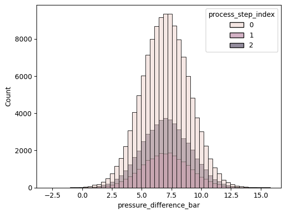
It appears like the pressure difference is roughly normally distributed and that the mean of the three processing steps is similar.
Absolute counts are visually harder to compare, so let us use relative frequencies instead and normalize each of the processing steps separately.
sns.histplot(
data=df_processes,
x="pressure_difference_bar",
hue="process_step_index",
bins=50,
common_norm=False,
stat="percent",
) # common_norm is set to False to normalize each processing step separately, stat is set to "percent" to show relative frequencies in percent.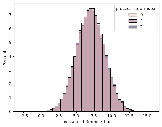
Apparently the pressure difference shares similar mean and standard deviation across the three processing steps. We can also show this by calculating the mean and standard deviation of the pressure difference for each processing step.
df_processes.groupby("process_step_index")["pressure_difference_bar"].mean()process_step_index
0 6.992650
1 6.990845
2 7.007579
Name: pressure_difference_bar, dtype: float64df_processes.groupby("process_step_index")["pressure_difference_bar"].std()process_step_index
0 1.990051
1 1.997792
2 2.015344
Name: pressure_difference_bar, dtype: float64We conclude that the pressure is not perfectly controlled (or measured) and have a systematic offset of 7 bar and a standard deviation of roughly 2 bar.
fig = px.line(
df_processes.sample(10_000).sort_values(
"timestamp"
), # for performance reasons, we sample 10,000 rows. Always remember to sort by timestamp after sampling.
x="timestamp",
y=["machine_temperature_C", "air_temperature_C"],
labels={"value": "Temperature (°C)", "timestamp": "Timestamp", "variable": "Type"},
title="Machine and Air Temperature Over Time",
)
fig.show()We observe that the machine is in a cold state when the data collection starts and heats up to a more stable plateau, where it still seems to follow the shape of the air temperature.
20.4.5 Aggregating plots
We are looking at iterations of the same, identical process. Let us look at a plot where the processes overlap each other, colored by error code.
First, we create a new index which starts at 0 for each piece that is manufactured and counts each timestamp within that process step. This index will be useful for plotting the different process iterations on top of each other.
df_processes["process_inner_index"] = df_processes.sort_values("timestamp").groupby("nr_iteration").cumcount()# Merge error_code from df_inspections into df_processes based on 'nr_iteration'. This assigns an errorcode to the entire process iteration.
df_plot = df_processes.merge(df_inspections, left_on="nr_iteration", right_index=True, how="left")
fig = px.line(
df_plot,
x="process_inner_index",
y="pressure_measured_bar",
line_group="nr_iteration",
color="error_code",
title="Pressure per Iteration (Overlapped, Colored by Error Code)",
labels={
"process_inner_index": "Inner-process timestamp",
"pressure_measured_bar": "Pressure (bar)",
"error_code": "Error Code",
},
)
# Set opacity: 0.01 for 'OK', 0.5 for others
# Setting opacity is always a bit tricky. Setting it too low makes the lines almost invisble, setting it too high makes the plot too crowded.
# This settings were found in trial and error and work well for that case.
for trace in fig.data:
if trace.name == "OK":
trace.opacity = 0.01
else:
trace.opacity = 0.5
# Unselect NOK_2 and NOK_3 by default, since they are very rare and would clutter the plot.
for i, trace in enumerate(fig.data):
if trace.name in ["NOK_2", "NOK_3"]:
fig.data[i].visible = "legendonly"
fig.update_layout(showlegend=True)
fig.show()Keep in mind that you can (de)select lines to plot when clicking on the according legend entry. Plotly also allows you to zoom in and pan around.
From the plot, we can see that the second processing step’s pressure is elevated for NOK_1. NOK_4 shows no obvious difference to OK.
With this in mind, let us have a closer look at the mean pressure and its standard deviation per error code and processing step.
# Aggregate: mean and std for each process_inner_index and error_code
agg_df = (
df_plot.groupby(["process_inner_index", "error_code"])["pressure_measured_bar"].agg(["mean", "std"]).reset_index()
)
fig = px.line(
agg_df,
x="process_inner_index",
y="mean",
color="error_code",
error_y="std",
labels={
"process_inner_index": "Inner-process timestamp",
"mean": "Pressure (bar)",
"error_code": "Error Code",
},
title="Mean Pressure per Error Code with Deviation",
)
# Unselect NOK_2 and NOK_3 by default
for i, trace in enumerate(fig.data):
if trace.name in ["NOK_2", "NOK_3"]:
fig.data[i].visible = "legendonly"
fig.update_layout(legend_title_text="Error Code")
fig.show()This plot confirms our previous observation that NOK_1 has a systematic higher mean pressure during the second processing step and NOK_4 does not differ notably from OK.
While the first line plot shows every individual process iteration as a singe line and therefor does not accidentally filter relevant information, it is a bit crowded and hard to read. The second plot aggregates the individual lines by calculating the mean and standard deviation, therefore losing some information, but making it easier to comprehend.
Now let us also check whether the machine temperature has an influence on failures.
df_agg = df_plot.groupby(["nr_iteration", "error_code"])["machine_temperature_C"].agg(["mean"]).reset_index()
fig = px.box(
df_agg,
x="error_code",
y="mean",
title="Machine Temperature by Error Code",
labels={"mean": "Mean Machine Temperature (°C)", "error_code": "Error Code"},
)
fig.show()Also here, NOK_4 and NOK_1 do not show a notable difference to OK, while NOK_2 and NOK_3 can not be judged well due to the low sample size.
20.4.6 Summary of findings
Let us summarize our findings so far in this dataset:
- The pressure during the second processing step is elevated for
NOK_1compared toOK. - The machine temperature does not show a notable difference between
OKandNOK_x. - The source of
NOK_4failures was not identified in this analysis. - The error codes
NOK_2andNOK_3are too rare to draw any conclusions.
Chapter 22 will dive deeper into the data and guide you through the process of optimizing the manufacturing process based on these findings.