In many real scenarios, data is acquired by manual input or when a certain event occurred, leading to irregular time steps.
Finding patterns in time series data is usually easier when time series have constant time steps. Some common time series methods, such as ARIMA or Recurrent Neural Networks, even require constant time steps.
When time series have irregular time steps, we can resample them to a regular frequency. To illustrate this, we generate a synthetic time series with irregular time steps and resample it to a regular frequency.
25.1 Example
25.1.1 Load packages
Code
import datetimeimport numpy as npimport pandas as pdimport matplotlib.pyplot as pltimport plotly.express as pximport plotly.io as pio # used to set the default plotly rendererpio.renderers.default = ("notebook"# set the default plotly renderer to "notebook" (necessary for quarto to render the plots))
25.1.2 Data Generation
Generate synthetic time series with irregular time steps.
Code
np.random.seed(42)n_steps =1000# Generate irregular time stepsstart_time = pd.Timestamp("2025-09-25 12:43:00")time_steps = pd.date_range(start=start_time, periods=n_steps, freq="1ms")# Use a sinus curve instead of a random walkfrequency =16.667# Hz# Calculate elapsed time in seconds for each time stepelapsed_seconds = (time_steps - start_time).total_seconds()values = np.sin(2* np.pi * frequency * elapsed_seconds)# Create a pandas Seriesdf_sinus = pd.Series(data=values, index=time_steps)df_sinus_sampled = df_sinus.sample(frac=0.2).sort_index()
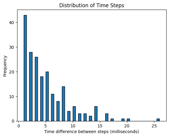
Using a histogram, visualizing the difference between consecutive time steps, we can see that time steps are not constant.
# Calculate time differences in seconds between consecutive time stepstime_diffs = df_sinus_sampled.index[1:] - df_sinus_sampled.index[:-1]time_diffs_seconds = time_diffs.total_seconds() *1000plt.hist(time_diffs_seconds, bins=50, edgecolor="k")plt.xlabel("Time difference between steps (milliseconds)")plt.ylabel("Frequency")plt.title("Distribution of Time Steps")plt.show()
25.1.4 Choosing a sampling frequency
Resampling ensures constant time steps, but usually requires some sort of alignment.
This can be done by oversampling (increasing the frequency) or undersampling (decreasing the frequency). Using a fixed frequency, the question arises, which value should be used for values at the newly introduced time step.
For undersampling, we usually have multiple values between two consecutive time steps of the resampled time series. This can be handled by aggregation functions, such as mean, median, min, max, sum, last value, next value, etc.
For oversampling, we usually have no value at the newly introduced time steps, which requires some form of interpolation.
resample_freq =5# millisecondsdf_sinus_resampled = df_sinus_sampled.resample(f"{resample_freq}ms").median().interpolate(method="pchip")df_sinus_resampled.index +=+datetime.timedelta( milliseconds=(resample_freq /2)) # pd.resample is not center-aligned; adjust for thatfig = px.line( x=df_sinus.index, y=df_sinus.values, labels={"x": "Time", "y": "Value"}, title="Lineplot of original data",)fig.add_scatter( x=df_sinus_sampled.index, y=df_sinus_sampled.values, mode="markers", name="sampled Points", marker=dict(color="red", size=6),)fig.add_scatter( x=df_sinus_resampled.index, y=df_sinus_resampled.values, mode="markers", name="resampled Points", marker=dict(color="green", symbol="x", size=6),)fig.show()