21 Process optimization via Live Feedback

In this section, we will have a look at a simulated example of a live feedback system in an industrial manufacturing context.

21.1 Setting the stage

Imagine a pick-and-place machine in a manufacturing line that is responsible for placing components onto a circuit board. The machine has two axes (X and Y) to position the placement head accurately over the board and a vacuum system to pick up and release components. Additionally it has a camera system to verify the placement accuracy of each component once it is placed. A couple of sensors provide real-time measurements and variables that can be used to monitor the process.

Unfortunately, the machine seems to be experiencing some issues with placement accuracy, leading to an increased number of defective boards. To address this, the engineers set up sandboxing mode where the machine performs four steps:

Move to pick up a component with random weight placed at a random location.
Pick up the component using the vacuum system.
Move to the target placement location on the circuit board with random speed. This is always at the center of the board at (150, 150).
Place the component and measure the placement accuracy using the camera system.

Until the end of step 2, it is possible to adjust the placement parameters by providing a correction vector that modifies the target placement location.

The goal is to optimize the placement parameters in real-time based on the feedback received from the camera system after each placement.

21.2 Accessible variables

The following variables are accessible during the process:

Air temperature [K]: ambient temperature around the machine.
Attached Weight [mg]: weight of the component picked up by the vacuum system.
Cycle: unique identifier for each cycle.
Error x [mm]: placement error in \(x\) direction (only available at the end of the cycle).
Error y [mm]: placement error in \(y\) direction (only available at the end of the cycle).
Position x [mm]: target position in \(x\) direction.
Position y [mm]: target position in \(y\) direction.
Process step: current step in the process (0 to 3).
Process temperature [K]: temperature inside the machine.
Speed [mm/s]: speed of the current movement.
Speed next [mm/s]: speed for the next movement.

21.3 Data

One cycle usually takes 3-6 seconds to complete and the sensor data is available in realtime via OPC Unified Architecture (OPC UA).

Note

OPC UA is a cross-platform, open-source communication protocol for data exchange in the industrial automation space developed by the OPC Foundation. It is a client-server architecture that allows for secure and reliable data transfer between devices and systems from different manufacturers.

Luckily, the engineers already collected a dataset of 25.000 cycles coming in two files:

simulated_opcua_machinedata.csv stores the sensor data.
simulated_opcua_postinspection.csv stores the placement error data.

The two datasets can be merged via cycle column.

21.4 Loading packages

import pandas as pd  # used for data handling
import seaborn as sns  # used for statistical data visualization
import plotly.io as pio  # used to set the default plotly renderer

pio.renderers.default = (
    "notebook"  # set the default plotly renderer to "notebook" (necessary for quarto to render the plots)
)

21.5 Loading the dataset

The dataset was released alongside the simulated machine at Ehrensperger (2026), but you can also clone the repository directly from GitHub. In this section, we will look at the provided csv files.

df_machinedata = pd.read_csv(
    "https://raw.githubusercontent.com/noxthot/industrial_datascience_live_machine/refs/tags/v1.0.0/data/simulated_opcua_machinedata.csv"
)
df_postinspection = pd.read_csv(
    "https://raw.githubusercontent.com/noxthot/industrial_datascience_live_machine/refs/tags/v1.0.0/data/simulated_opcua_postinspection.csv"
)

21.5.1 Data integrity check

df_machinedata

	Air temperature [K]	Attached Weight [mg]	Position x [mm]	Position y [mm]	Process step	Process temperature [K]	Speed [mm/s]	Speed next [mm/s]	timestamp	cycle
0	24.755379	0.000000	191.828040	7.503227	0	30.385614	100.000000	0.000000	2026-01-08T13:37:00	1
1	25.215286	223.987527	191.828040	7.503227	1	31.615630	0.000000	34.752639	2026-01-08T13:37:01.505090	1
2	24.666009	223.987527	150.000000	150.000000	2	31.998852	34.752639	0.000000	2026-01-08T13:37:02.025090	1
3	25.115265	0.000000	150.000000	150.000000	3	33.046526	0.000000	100.000000	2026-01-08T13:37:06.318405	1
4	25.129309	0.000000	7.960791	59.651295	0	33.194048	100.000000	0.000000	2026-01-08T13:37:06.338405	2
...	...	...	...	...	...	...	...	...	...	...
99995	8.068273	0.000000	150.000000	150.000000	3	17.642248	0.000000	100.000000	2026-01-09T21:57:12.230277	24999
99996	10.301384	0.000000	273.977920	126.801859	0	16.803874	100.000000	0.000000	2026-01-09T21:57:12.250277	25000
99997	9.924715	193.867063	273.977920	126.801859	1	16.295092	0.000000	27.812182	2026-01-09T21:57:13.531573	25000
99998	9.452700	193.867063	150.000000	150.000000	2	16.074561	27.812182	0.000000	2026-01-09T21:57:14.051573	25000
99999	10.116288	0.000000	150.000000	150.000000	3	17.222515	0.000000	100.000000	2026-01-09T21:57:18.606622	25000

100000 rows × 10 columns

df_postinspection

	cycle	error_x	error_y
0	1	-0.192236	0.654895
1	2	1.285577	0.817733
2	3	-0.456091	0.163004
3	4	-1.734704	-0.624146
4	5	-0.496285	0.494395
...	...	...	...
24995	24996	1.080388	2.691526
24996	24997	-0.566057	-0.794911
24997	24998	-0.580030	0.738004
24998	24999	0.773854	-1.404837
24999	25000	-0.842577	0.157659

25000 rows × 3 columns

df = df_machinedata.merge(df_postinspection, on="cycle", how="left")
df

	Air temperature [K]	Attached Weight [mg]	Position x [mm]	Position y [mm]	Process step	Process temperature [K]	Speed [mm/s]	Speed next [mm/s]	timestamp	cycle	error_x	error_y
0	24.755379	0.000000	191.828040	7.503227	0	30.385614	100.000000	0.000000	2026-01-08T13:37:00	1	-0.192236	0.654895
1	25.215286	223.987527	191.828040	7.503227	1	31.615630	0.000000	34.752639	2026-01-08T13:37:01.505090	1	-0.192236	0.654895
2	24.666009	223.987527	150.000000	150.000000	2	31.998852	34.752639	0.000000	2026-01-08T13:37:02.025090	1	-0.192236	0.654895
3	25.115265	0.000000	150.000000	150.000000	3	33.046526	0.000000	100.000000	2026-01-08T13:37:06.318405	1	-0.192236	0.654895
4	25.129309	0.000000	7.960791	59.651295	0	33.194048	100.000000	0.000000	2026-01-08T13:37:06.338405	2	1.285577	0.817733
...	...	...	...	...	...	...	...	...	...	...	...	...
99995	8.068273	0.000000	150.000000	150.000000	3	17.642248	0.000000	100.000000	2026-01-09T21:57:12.230277	24999	0.773854	-1.404837
99996	10.301384	0.000000	273.977920	126.801859	0	16.803874	100.000000	0.000000	2026-01-09T21:57:12.250277	25000	-0.842577	0.157659
99997	9.924715	193.867063	273.977920	126.801859	1	16.295092	0.000000	27.812182	2026-01-09T21:57:13.531573	25000	-0.842577	0.157659
99998	9.452700	193.867063	150.000000	150.000000	2	16.074561	27.812182	0.000000	2026-01-09T21:57:14.051573	25000	-0.842577	0.157659
99999	10.116288	0.000000	150.000000	150.000000	3	17.222515	0.000000	100.000000	2026-01-09T21:57:18.606622	25000	-0.842577	0.157659

100000 rows × 12 columns

21.6 Error Visualization

sns.jointplot(data=df_postinspection, x="error_x", y="error_y", kind="kde", fill=True, cmap="viridis")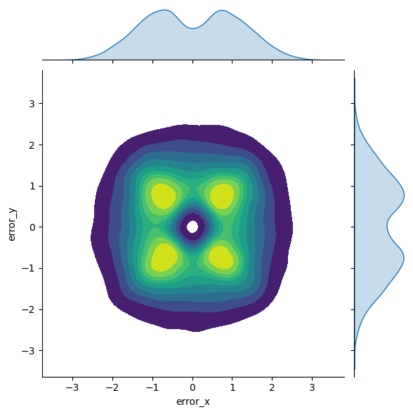

This is a rather interesting error distribution.

21.7 Next Steps

Chapter 23 will guide you through the optimization process aimed at reducing these errors and improving overall process accuracy.